Introduction to the Spark BigQuery connector

We recently described some technical details about Spark and BigQuery. BigQuery is a powerful data warehouse and can work as an analytics platform or even for training machine learning models. However, not every data pipeline can be described with SQL. Another option for defining a data transformation is a Spark job. In this post, we’ll show you how you can connect these two powerful tools to access BigQuery tables and load data into Spark applications, thereby addressing even more intricate challenges in the realm of data science. Later, we will discuss in detail how reading from BigQuery into Spark works and what are the main tips and tricks to lower the cost* of a pipeline.

*When we talk about the cost of BigQuery Analysis we use on-demand pricing, not capacity pricing.

Basics

BigQuery is a Google Cloud Platform service, and it's not surprising that the library enabling data exchange between Spark and BigQuery is maintained by Google developers. If you want to look at the source code of the connector it is publicly available on GitHub - spark-bigquery-connector. Before using the connector, please note that there are two main versions: 

• Older: com.google.cloud.spark:spark-bigquery-with-dependencies_{scala_version}
• Newer: com.google.cloud.spark:spark-{spark_version}-bigquery

For exact versions please refer to the connector’s README.

The Spark BigQuery connector is now a built-in feature of Dataproc image versions 2.1 and above, simplifying the process and making it unnecessary to manually provide the connector yourself. This means you no longer have to worry about specifying it with --jars or --packages flags.

If you need to use a specific version of the connector other than the built-in one, you can override it during cluster or batch creation by adding a metadata or properties flag. For example, to specify a different version for a Dataproc cluster, you can use the --metadata SPARK_BQ_CONNECTOR_VERSION=0.42.2 flag (see Figure 1.).

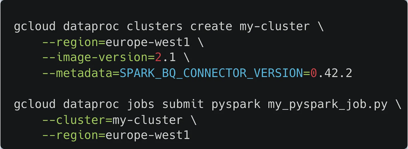
First, we create the cluster and override the built-in connector by using the --metadata flag. Since the connector is already configured on the cluster, we can submit our PySpark job directly without needing to provide the JAR file with the --jars flag.

How to read data from Google BigQuery?

Before reading the data from BigQuery tables, we need to distinguish between reading partitioned and standard tables. When it comes to partitioned tables in most cases we only want to read a limited number of partitions. Reading all partitions is very rare. That's why we need to select an additional filter that specifies only these partitions that we need (see Figure 2.). By utilising the filter option, data will be filtered directly on BigQuery and never read to the Spark cluster. In contrast, standard tables are often read at once and we could omit additional filters (see Figure 3.). The connector operates by utilising the BigQuery Read Storage API, allowing seamless direct data retrieval from BigQuery storage. This eliminates the necessity of exporting data to temporary CSV, parquet, AVRO files, or executing supplementary queries.

Condition on a _PARTITIONDATE pseudo column BigQuery sends only selected partitions to the Spark cluster.

Can you access a partitioned table without utilising the `_PARTITIONTIME` filter? Indeed, it's feasible, but it comes with significant risks. If you've deactivated the BigQuery table option "require partition filter," you can read the entire table just like a standard table, as shown in Figure 3. - the entire table! This means there won't be any filtering on the BigQuery side. All partitions will be fetched by Spark, and a substantial portion of them is likely to be discarded. Consequently, you'll incur charges for all the data read, even if it's not essential for subsequent processing. Our strong recommendation is to always activate the "require partition filter" option.

Reading data using Spark SQL query

If you look into the Spark BigQuery connector documentation you can find information about another option - reading via SQL query. It is a very powerful option, but a user should have considerable knowledge of how this option works. I hope that after this paragraph you will understand why using queries such as “SELECT * FROM `table`” in that context is a very bad idea.

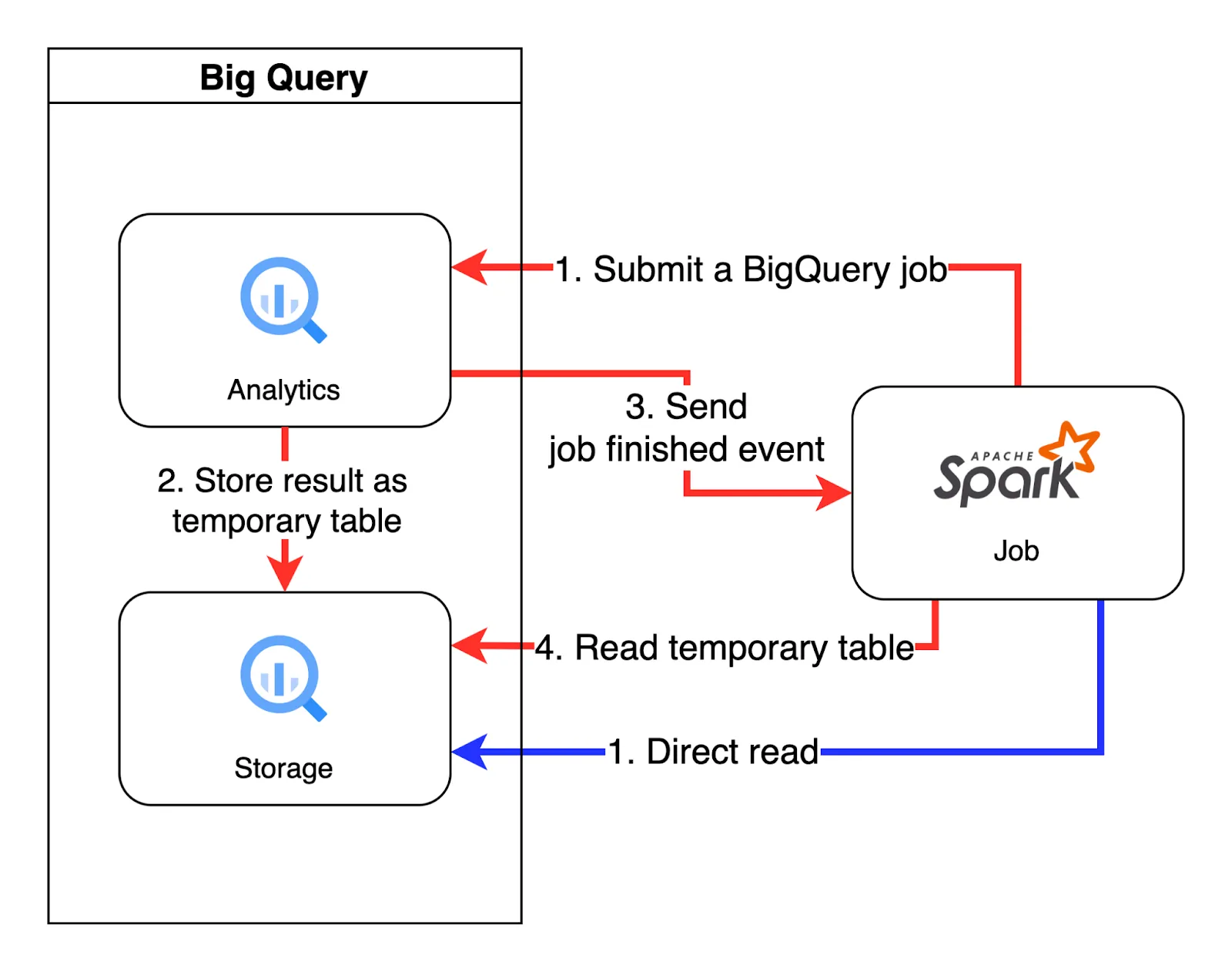
Reading data from BigQuery to the Spark with SQL query has two stages:

1. Application submits SQL to BigQuery. Results are saved into a “temporary” table in BigQuery.
2. Spark reads data from the “temporary” table into the cluster.

Of course, every step is billed separately. Keeping in mind that when using on-demand pricing, running a job on BigQuery costs approximately five times more than reading data with BigQuery Storage API. However, this additional BigQuery job can cut costs significantly by reducing the processing load on the Spark cluster. We will talk more about when it can be helpful later. For now let’s just show how it is done.

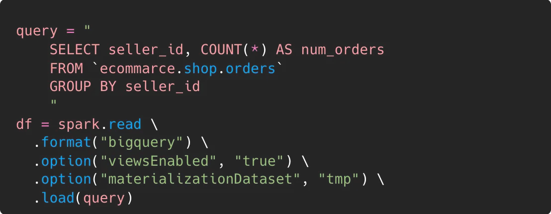
There are two additional things that we need to initially specify. First of all we need to set option `viewsEnabled` to true. Reading via SQL is very similar to reading from views. It requires running additional jobs on BigQuery. This flag is confirmation that a user knows that this will come with additional costs. The second one is an option `materializationDataset`. That’s the dataset where the “temporary” table will be created. The table will be available in the materialisation dataset by default for one day. You can modify that time by using the materializationExpirationTimeInMinutes option, but setting very low values can lead to some inconsistency as can be read in the Spark BigQuery connector documentation. Having everything set correctly, we can run our pipeline (see Figure 4.).

‍

When monitoring the real-time execution of the job, you may observe that nothing appears to happen until the first Spark query is submitted. Typically, Spark requires some time to prepare and optimise the execution plan. However, when utilising the "query" option, this time may be prolonged, as queries are executed immediately upon reaching that line in a script. This might seem counterintuitive, as loading is typically part of the Spark plan. It's essential to remember that the query represents an additional step before executing the Spark load method.

If your job seems to be stuck, it's advisable to check the BigQuery console and look for the currently running query. We encountered a situation where a query had been running for half an hour, while the Spark cluster was waiting for the result and remained idle. This drawback of the method results in the waste of cluster time, which is often associated with usage costs.

There is one more small disadvantage of that method, but only for those that have a physical storage billing model. You will pay for some time for storing that table even if it has been deleted. There are two safety features after the table / partition in BigQuery is deleted: time travel and fail-safe. Both are paid in a physical storage model even though you will rarely need to restore “temporary” connector tables. A little improvement might be modifying time travel in a materialisation dataset and setting it to minimal value (two days). 

To sum up we have prepared a chart (see Figure 5.) that shows the main differences between reading data directly from BigQuery storage and with the usage of additional queries. The general rule of thumb is to use direct reading, because it is usually cheaper and faster.

Column and predicate filtering

Nearly everything on GCP costs, reading data from BigQuery is no exception. When building data pipelines optimization takes on a new context. The amount of data read not only affects time needed to process that data but also defines how much we would pay for moving it out of BigQuery. The good news is that the Spark BigQuery connector can help with both column and predicate filtering.

We don’t usually need to load all columns of a particular table to a spark dataframe. BigQuery has a columnar storage format and can effectively return only columns that are needed for later processing. The connector analyses the Spark query plan and sends a request to BigQuery to read only necessary columns from a table. However, pay attention to the version of Spark BigQuery connector that you are using.  For older connector versions pushdown of predicate filtering does not work for nested fields (see Figure 6.). It was upgraded in version 0.34.0 - PR #1104.

If we can filter columns then maybe we can filter rows as well? The answer is yes, but in practice once again there is a problem with nested columns. Simple filters like checking equality or less/greater than are pushed down. However, when it comes to the nested columns - filters are not pushed down. It was reported by our colleague Michał Misiewicz as issue #464. Connector maintainers pointed out that it is possible to specify additional conditions in the option filter. That’s the same option that we have been using to select particular partitions in a previous section. That’s not ideal, but at least we have an option.

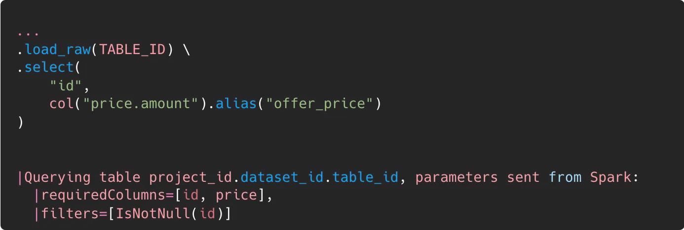
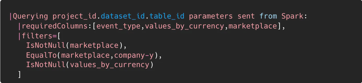
From theory to practice, How can I check if column and predicate filtering is working? The easiest way is to check the application logs. Whenever the Spark BigQuery connector opens a new read session logs with read schema and pushed down filters are emitted (see Figure 7.).

‍

This connector can even optimise empty projections like finding a number of rows in a table (see property - optimizedEmptyProjection). In that case the connector would read that number from the table metadata.

BigQuery jobs to the rescue!

As we showed earlier, reading data through SQL query can incur additional costs. However, sometimes it turns out using it might reduce the overall cost of running the whole data pipeline. 

By default BigQuery offers 1,000 slots (~500 CPU)  that can process our data. In contrast Spark clusters size in most cases does not exceed 100 CPU so BigQuery can process the same data faster, for example calculate aggregate of large dataset. That’s the first scenario where off-loading data processing might be cost effective. We pay for an additional job on BigQuery, but it reduces overall cluster lifetime. Sometimes it could even shrink the cluster size, because the amount of read data has decreased.

Some time ago we found that reading a small partitioned table (~30MB in total), but split into thousands of partitions works poorly. In our case, reading data from that particular table took 10 minutes. We came up with an idea that gathering that partition into one block and then reading it into the Spark cluster would speed up the whole process. Indeed, when we run the query that reads the entire table and stores it into a “temporary” table, the time needed to read the table decreases from 10 minutes to under 5 seconds (see Figure 8). The cost of the additional query was marginal as the data volume was very low, but we saved up 10 minutes of cluster time. Keep in mind that our entire task can be accomplished in just 20 minutes, so reducing it by 10 minutes equates to a 50% reduction in cluster costs! 

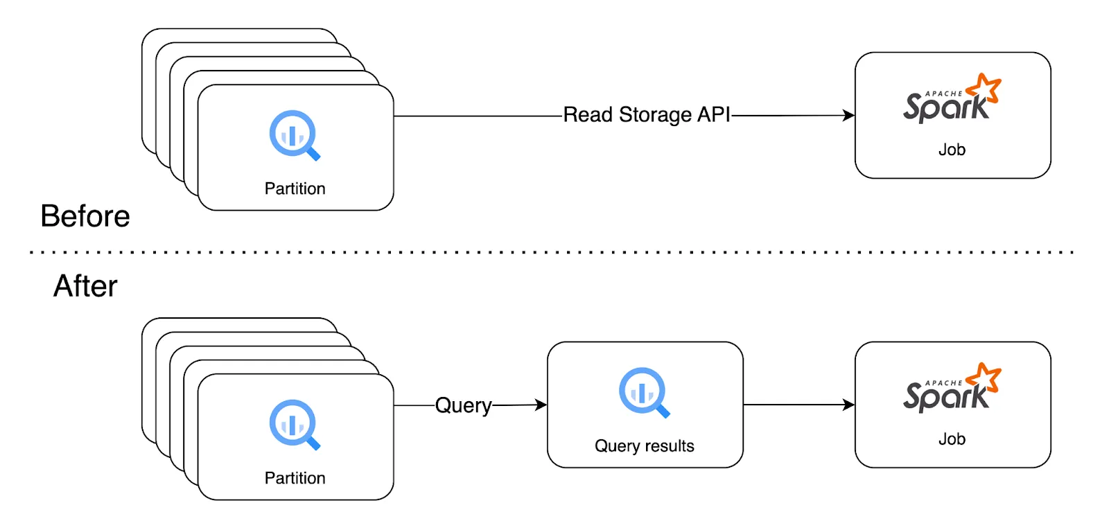
Figure 8. With additional SQL query we collected multiple partitions into one ‘temporary’ table. As a result the time needed for reading the whole dataset decreased from ~10 min to <5 sec. 

Read parallelism

For us the most important feature of BigQuery Storage API is its ability to handle multiple streams in one session. In practice it allows each Spark executor to read its portion of data from BigQuery simultaneously. There are two parameters to control parallelism: `maxParallelism` and `preferredMinParallelism`.  The `maxParallelism` is an upper bound, where `preferredMinParallelism` is a lower bound of concurrent reads. However, the actual number of chunks might be lower if the dataset is small. The default for the `preferredMinParallelism` is 3 x spark.default.parallelism. For `maxParallelism` it is 20 000. In most cases you do not need to change these parameters, but we faced some situations where tuning it helped.

Spark works well when a partition size is around 300-400 MB. When partitions are smaller we waste time on task scheduling. When partitions are larger there are often problems with spill to disk and GC. In most cases BigQuery does a good job when it comes to finding the right number of partitions for small datasets. However, sometimes it might be helpful to set `maxParallelism` if we observe many small partitions during the reading. On the other hand, reading a large dataset requires splitting it into smaller partitions. Increasing the `preferredMinParallelism` parameter could help overcome this.

Conclusion

Google BigQuery and Apache Spark could work together to face more challenging tasks and enable building robust data pipelines. To analyse BigQuery data, the first step is always to read the data from the warehouse. A good data engineer should have at least basic knowledge of what tools could be used to achieve that. Spark BigQuery connector offers plenty of options and configuration properties. In this blog we discussed only the most important. Also we see that Connector still has its downsides. However, it is actively being developed and it might turn out that some of its shortcomings may be ironed out soon.

Image credentials

Intro - Generated with AI - Bing Image Creator ∙ 11 December 2023